
State space models using JAGS in R
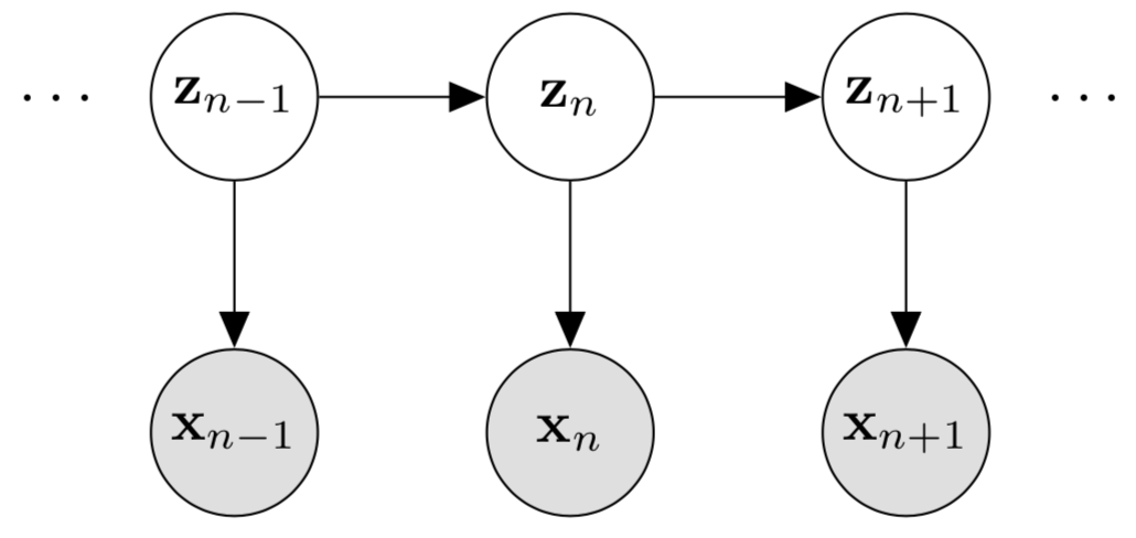
A hidden markov model, figure source here
Introduction
Models with unobserved components are frequently encountered in ecology. These processes may be modelled with the help of state-space models that provides a way of modelling dynamic systems. These models avoid the need to use proxy variables for the unobservable variables, thus avoiding biased parameter estimates. State space models are a kind of autoregressive (i.e., use past to predict future) time series model, but instead of having an arbitrary number of autoregressive components (e.g., lags of weeks, months, or years), it uses a single first order autoregressive component i.e., only use the information from the previous time step. It allows to incorporate uncertainty in the observation process; by independently modelling the process model (how the system actually changes) and the observation model (how the system is observed under the underlying process). State space models are also described as hidden Markov models (HMMs) and latent process models.
If we consider, $y$: observed response variable and $X$: hidden state, then the process and the observation model can be represented mathematically as:
Process model
The actual response at time $t+1$ is a function of the actual response at time $t$ plus some error.
\[X_{t+1} = f(X_t) + \epsilon_t\] \[X_{t+1} = b_0 + b_1 X_t + \epsilon_t \;\;\;\;\; \epsilon_t ~ N(0, \sigma^2)\]Observation model
The observed response variable $y_t$ is a function of the hidden state and some error.
$y_t = X_t + \epsilon_t$ $\;\;\;\;\;$ $\epsilon_t$ ~ $N(0, \sigma^2)$
It can also be written as
$y_t$ = $N$($X_t$,$\;$$\sigma^2$)
where $X_t$ is the hidden state (the actual entity that we are interested), $y_t$ is the observed response variable, $f$ is the process model, $\epsilon_t$ is the process error, $\epsilon_t$ is the observation error, and $b_0$ and $b_1$ are the parameters of the process model.
Simulate and predict using JAGS in R
Let us consider a common example in Ecology i.e., the measure of population size of species. Often the population size is not directly observed, but is estimated from the number of individuals captured in a survey (e.g., count data). The number of individuals captured in a survey is a noisy estimate of the actual population size. The population size is a hidden state, and the number of individuals captured in a survey is the observed response variable. The process model is the population size at time $t+1$ is a function of the population size at time $t$, plus some error. The observation model is the number of individuals captured in a survey is a function of the population size and some error.
Lets start coding in R. First, we need to install the required packages. You will need to install jags (“Just another Gibbs Sampler”) in your system and rjags package in R to run the tutorial. Debian/Ubuntu users can install jags with the following command in the terminal:
sudo apt-get install jags
Then open R and install the rjags package:
install.packages("rjags")
Simulate the observed data and the hidden state, and let X: process model (actual population size) and y: observation model (observed species count)
#simulate data

set.seed(123)
N <- 100 # number of time points
r <- 1.03 # population growth rate

X <- rep(NA, N) # actual population size
X[1] <- 50 # set initial population size to 50
Y <- rep(NA, N) # observed species count

# define errors for process and observation models
sigma_proc <- 0.30 # process error
sigma_obs <- 100 # observation error

# assign values to X and y
for (t in 1:(N-1)) {
  X[t+1] <- X[t] * rnorm(N-1, mean = r, sd = sigma_proc)
  y[t] <- X[t] + rnorm(1, mean = 0, sd = sigma_obs)
}
Define a JAGS model (requires a string object)
model_string <- "
model {
  # Observation model
  for (t in 1:N) {
    y[t] ~ dnorm(x[t], tau_obs)
  }

  # Process model
  for (t in 2:N) {
    x[t] ~ dnorm(x[t-1], tau_proc)
  }

  # Priors
  tau_obs ~ dgamma(a_obs, r_obs) # prior for observation error
  tau_proc ~ dgamma(a_proc, r_proc) # prior for process error
  x[1] ~ dnorm(x_ic, tau_ic)  # prior for intercept
}
"
Create a data list object to pass to the JAGS model. The data list assigns the simulated data to the variables in the JAGS model.
data_list = list(
  y = y,
  N = N,
  x_ic = 100,
  tau_ic = 1,
  a_obs = 1,
  r_obs = 1,
  a_proc = 1,
  r_proc = 1
)

# x_ic pretend that you don't know the initial population size and
# estimate it to be 100 looking at the y series
Initial priors for the parameters of the model. These are the starting values for the MCMC algorithm.
init = list(list(tau_proc = 1/var(diff(y)), tau_obs = 1/var(y)))
Compile the model and run the MCMC algorithm. The jags.model function returns a jags object. The jags object contains the MCMC samples, the model, and the data. The jags object can be used to extract the MCMC samples, and to plot the MCMC chains.
# Compile the model
model <- jags.model(textConnection(model_string),
                    data = data,
                    inits = init,
                    n.chains = 1)
Run the MCMC sampler
samples <- coda.samples(
  model = model,
  variable.names = c("tau_proc", "tau_obs", "x"),
  n.iter = 10000)

#plot(samples) plot the chains
Extract the MCMC samples and plot
output <- as.matrix(samples) # extract the MCMC samples
only_Xs = output[ , 3: ncol(output)] # get only X values
pred <- colMeans(only_Xs) # point estimates and the variance
pred_interval <- apply(  # get 95% prediction intervals
  only_Xs, 2,
  quantile, c(0.025, 0.975))

# arrange in a dataframe
df <- df |>
  mutate(pred = pred,
         lpred = pred_interval[1,],
         upred = pred_interval[2,])


# plot the actual values, and predicted values and interval
p2 <- ggplot(df, aes(x = t)) +
  geom_ribbon(aes(ymin = lpred, ymax = upred), alpha = 0.3, fill = "gray") +
  geom_point(aes(y = y, col = "Observed count"), size = 2) +
  geom_line(aes(y = X, col = "Actual size"), linewidth = 1) +
  geom_line(aes(y = pred, col = "Predicted size"), linewidth = 1) +
  scale_color_manual(values = c("Observed count" = "red",
    "Actual size" = "#009B95", "Predicted size" = "#4B0055"), name = "") +
  labs(y = "No. of species", x = "time") +
  theme_minimal()

It looks like the model predicted the population size well (closely matching green and blue lines), although the predicted interval doesn’t look too promising, I think.
Forecasting
How well does the model forecast ? We can check that by splitting the y data, let’s remove the last 20 years of data and predict on those. The modelling process is similar to the previous one, except that we need to specify y in the mcmc sampler.
data$y[40:60] <- NA

# change the "x" from previous script to "y" in variable names
samples <- coda.samples(
  model = model,
  variable.names = c("tau_proc", "tau_obs", "y"),
  n.iter = 10000)
The predicted values are quite poor (almost a naive estimator), but it’s not unexpected given the not so complex model.
