
Point process modelling of forest fires using inlabru

Wildfires are among the important drivers of biodiversity and ecosystem loss globally. In order to gain insight into the potential impact of global warming and climate change on the environment in the future, it is essential to model the occurrence and size of wildfires, as well as to identify factors associated with their spatial distribution and burned area. Wildfires are influenced by their spatial location, timing, and related factors. While techniques such as Markov Random Fields can provide some useful information, spatial point processes are the preferred analytical method for studying the spatial and spatio-temporal patterns of forest fires.
In this blog post, I will demonstrate how to use inlabru a wrapper around the popular INLA (Integrated Nested Laplace Approximation) package to model the spatial distribution of forest fires using the CLM fires dataset. I am motivated by this blog, which uses INLA core and is much more detailed, I am using inlabru which does most of the work in the background and further, I have shortened up the code to look cleaner and concise. The INLA-SPDE approach has the benefit of being able to predict marginal distributions of both the model parameters and response, without conducting time-consuming simulations as in other bayesian approaches that use MCMC. The CLM fires dataset contains the locations fires in the Castilla-La Mancha region of Spain between 1998 and 2007. This region is approximately 400 by 400 kilometres. The dataset is available in the spatstat package in R.
We will model the response using a log-Gaussian Cox process (LGCP). A log-Gaussian Cox process is a type of stochastic model used to analyze spatial point patterns. It is a special case of a Cox process, which is a type of point process that models the intensity of points as a function of covariates. In a log-Gaussian Cox process, the intensity of the point process is assumed to be log-normally distributed, which allows for the incorporation of spatially dependent random effects.
The log-Gaussian Cox process is commonly used in environmental and ecological applications, such as modeling the spatial distribution of wildfire occurrences, disease outbreaks, or species distributions. It has the advantage of allowing for the modeling of complex spatial patterns, as well as the incorporation of spatially-dependent covariates and random effects. Mathematically, the log-Gaussian Cox process is defined as:
λ(x) = exp(β₀ + β₁x₁ + ... + βₚxₚ + Z(x))
where λ(x) is the intensity of the point process at location x, β₀ represents the intercept term and β₁, …, βₚ represent the coefficients of the predictor variables x₁, …, xₚ respectively, and Z(x) is a spatially dependent random effect. The spatially dependent random effect Z(x) is assumed to be log-normally distributed, which allows for the incorporation of spatially dependent random effects.
Additionally, the log-Gaussian Cox model is able to account for overdispersion in the data, which is often observed in point pattern data such as wildfire occurrences. This overdispersion occurs when there is more variation in the data than would be expected under a Poisson process, which assumes that the occurrence of events is independent and random.
INLA depends upon objects of class defined by sp package; which is a package for spatial data but is retiring soon. INLA has not been updated to work with the new sf and terra packages. Hopefully, we will see an update soon.
Since we need sp objects to model, it is also important to understand the structure of the sp objects, mainly they are:
- SpatialPointsDataFrame: a data frame with a spatial component. The spatial component is a SpatialPoints object, which is a list of coordinates. The coordinates are stored in a matrix with two columns, one for the x-coordinate and one for the y-coordinate.
- SpatialPixelsDataFrame, which is a data frame with a spatial component (it’s a raster equivalent of terra).
Load R packages
packages <- c("inlabru", "sf", "raster", "sp", "spatstat", "tidyverse", "scico", "cowplot")
purrr::map(packages, library, character.only = TRUE)
Load data and arrange
# data from spatstat package
data(list = c("clmfires","clmfires.extra"))

# covariate data (use elevation as an example)
X <- clmfires.extra$clmcov100$elevation |>
  raster() |> # convert to raster object first for scaling
  scale() # centering and scaling for better model fit

X_spdf <- X |>  # convert to SpatialPixelsDataFrame
  as("SpatialGridDataFrame") |>
  as("SpatialPixelsDataFrame")

# response data (fire points)
y <- clmfires[clmfires$marks$cause == "lightning", ] |>
  st_as_sf(coords = c("x","y")) |>
  drop_na() |>
  as_Spatial()

# region of interest / study area boundary
roi <- do.call(cbind, clmfires$window$bdry[[1]])

roi_bb <- roi |>
 as.data.frame() |>
 st_as_sf(coords = c("x","y")) |>
 st_combine() |>
 st_cast("POLYGON") |>
 as_Spatial()
Create a Stochastic Partial Differential Equations (SPDE) mesh for the spatial random effects
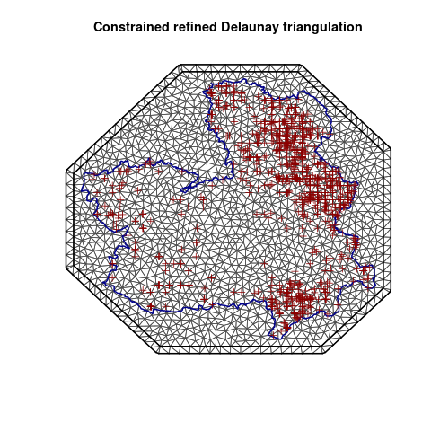
The SPDE mesh is a discretization of the continuous spatial domain into a set of connected triangles or polygons, where each triangle or polygon is defined by a set of nodes and edges. The nodes are points where the value of the spatial process is estimated or observed, while the edges connect the nodes and define the neighborhood structure of the mesh. The mesh is used to create a spatial covariance matrix, which is used to model the spatial dependence of the random effects. Moreover, SPDE mesh allows efficient representation of the spatial domain, regularise the spatial process, to reduce noise and overfitting in the model, helps in efficient computation of the posterior distribution using sparse matrix techniques, greatly reducing the computational costs of the model.
# Create a two dimensional spatial domain

mesh <- INLA::inla.mesh.2d(
            loc.domain = roi,
            max.edge = c(15, 30),
            offset = c(10, 10))

# Arguments:
#1. loc.domain specifies the domain of interest as a rectangular region
#2. max.edge specifies the maximum edge length of the mesh in each
# dimension, in our case, 15 and 30 means x-dimension should be
# max of 15 units and y-dimension should be max of 30 units.
#3. offset specifies the offset of the mesh from the boundary -
# to avoid numerical issues, in our case add 10 units to
# both x and y coordinates.
# plot the mesh
plot(mesh)
plot(roi_bb, border = "darkblue", lwd = 2, add = TRUE)
plot(y, col = "darkred", add = TRUE)
Define the priors for a Matérn class SPDE model
matern <- INLA::inla.spde2.pcmatern(
  mesh,
  prior.sigma = c(50, 0.9),
  prior.range = c(1, 0.01)
)

# Arguments:
#1. mesh: is the SPDE mesh we created above
#2. prior.sigma: specifies the prior distribution on the spatial precision
# parameter of the Matérn model. The precision parameter is the inverse of
# the variance, and it controls the amount of spatial variation in the model.
# In this example, prior.sigma = c(50, 0.9) specifies a normal prior
# distribution with a mean of 50 and a standard deviation of 0.9 on the
# logarithm of the spatial precision.
# 3. prior.range: species priors on the range parameters and determines
# the spatial correlation of the process, first vector is the mean of the
# range parameter and the second vector is the standard deviation of the
# range.
Create the model with the covariate
model <- coordinates ~ X_spdf +
  spde(coordinates, model = matern) -
  Intercept(1)
Fit the model using inla
fit <- lgcp(
  model,  # defined model from above
  y, # response data
  samplers = roi_bb, # sample only from region of interest
  domain = list(coordinates = mesh),
  options = list(control.inla = list(int.strategy = "eb"))
)

# eb = empirical Bayes for numerical integration of LGCP likelihood
The fit object is a list that includes the estimated parameters of the model, the intensity function, which represents the expected number of fires within a unit area, among others.
You can investigate the model fit and parameters using the summary() function.
summary(fit)
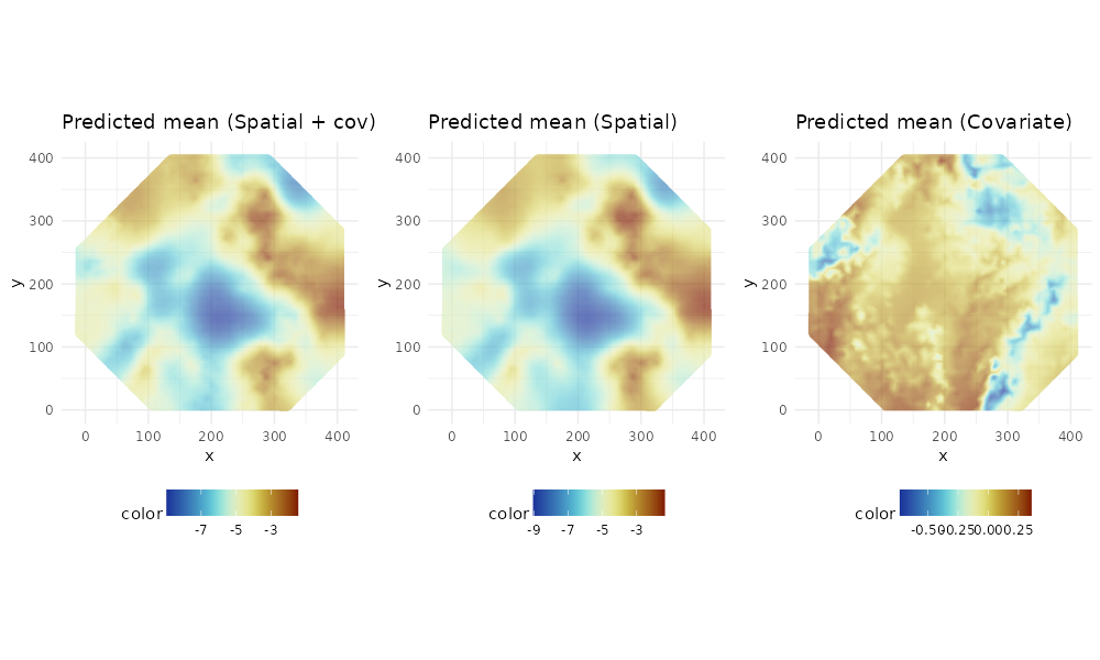
Predict the SPDE and the covariate at the mesh vertex locations
# get the vertices
vertices <- vertices.inla.mesh(mesh)
# plot(vertices)

# predict on the vertices
pred <- predict(
  fit,
  vertices,
  ~ list(
    joint = spde + X_spdf,
    field = spde,
    cov = X_spdf
  )
)
Plot the predicted intensity function
#Color scheme from scico (color blind friendly)
pal_a <- scico::scico(n=1000, palette = "roma", direction = -1)

p1 <- ggplot() +
  gg(mesh, color = pred$joint$mean) +
  coord_equal() +
  labs(title = "Predicted mean (Spatial + cov)") +
  scale_fill_gradientn(colors = pal_a) +
  theme_minimal() +
  theme(legend.position = "bottom")

p2 <- ggplot() +
  gg(mesh, color = pred$field$mean) +
  coord_equal() +
  labs(title = "Predicted mean (Spatial)") +
  scale_fill_gradientn(colors = pal_a) +
  theme_minimal() +
  theme(legend.position = "bottom")


p3 <- ggplot() +
  gg(mesh, color = pred$cov$mean) +
  coord_equal() +
  labs(title = "Predicted mean (Covariate)") +
  scale_fill_gradientn(colors = pal_a) +
  theme_minimal() +
  theme(legend.position = "bottom")

p <- cowplot::plot_grid(p1, p2, p3, nrow =1)

ggsave("intensity.png", p,
  width = 10, height = 6,
  units = "in", dpi = 100,
  bg = "white")
Final note: modelling is difficult; and even more for fires
While setting up and fitting the model is easy to implement, thanks to inlabru, the modelling process is itself not easy. There are a range of decisions that will affect the model performance and the results. These include variable selection, as the improper use may result in different model parameters and wrong interpretation of the system. Variable selection can be done with different methods e.g., step-wise backward selection (which are a bit criticized in literature). I love DAGs proposed by Judea Pearl- I am familiar with using DAGs for the non-spatial models but I have not yet implemented these in spatial models, so this is something that I will try to do in the future. Here is quickie on DAGS. Moreover identifying and selecting the appropriate covariates for fire modelling is challenging; as it’s quite a complex system with many interacting factors including fuel load, soil moisture, wind, temperature, and many others.
Other choices include: the choice of the prior distributions for the parameters for the covariance and the covariate effect (the different X beta’s), the choice of the spatial covariance function, the choice of the spatial mesh, the choice of the numerical integration method, the choice of the optimization method, the choice of the sampling method, and many others. So before modelling, it is important to have a good understanding of the system and the data these include making extra effort in exploratory data analysis. Another good practice is to use different models and compare them using different model selection criteria e.g., goodness of fit metrics like the Deviance Information Criterion (DIC) and the Watanabe-Akaike information criterion (WAIC).
I hope you enjoy this post and find it useful. If you have any questions or comments, please feel free to reach out to me on twitter or via email.