Deep learning using tensorflow/keras

Deep learning using tensorflow/keras

Introduction

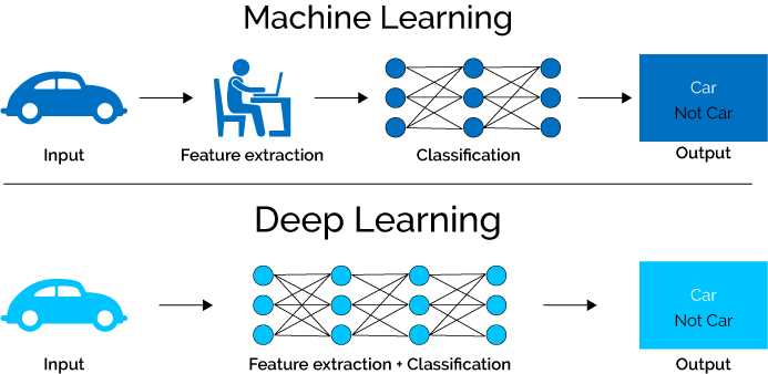
A Deep Neural Network (DNN) is simply an Artificial Neural Network (ANN) with one or more hidden layers. The hidden layers are the layers between the input and output layers. The more hidden layers a DNN has, the deeper it is. The deeper a DNN is, the more complex the functions it can learn. ANNs uses interconnected nodes or neurons in a layered structure that resembles the human brain.

A major difference between other machine learning techniques and ANNs is that ANN’s can learn the best features and their combinations, i.e., they can perform feature engineering themselves, in constract to other machine learning algorithms that require manual feature engineering. ANNs are more useful for unstructured data (those that can’t be easily put into a table e.g., images, text, audio, video, etc), where conducting manual feature engineering can be challenging. But ANN’s can also be used for structured/tabular data.

But there is a catch: the results are not easily interpretable. So if you are modelling species distribution, and you don’t care about why the model predicts the probability of a species to be present in a given area, then you can use a deep neural network.

The structure of the model is quite simple, each connection from one neuron to another has an associated weight (w), which is a measure of the strength of the connection. Each neuron (except the input layer) has an extra weight called as the bias weight (b). These weights are the parameters that are learned during training (Actually, learning in neural network is nothing but the the adjustment of these weights). The weight is multiplied by the input value and the results are summed to produce the input to the neuron. The input is then passed through an activation function to produce the output of the next neuron.

NNs are trained by using gradient descent algorithm to minimise the loss function (see this nice and short tutorial) and applying weight updates incrementally via backpropagation to minimise the loss or cost. The most important feature in an activation function is its ability to add non-linearity into a neural network. Without non-linearity and activation function, a neural network is just a linear regression model.

Common activation functions are:

(i) Sigmoid or logistic: an ‘S’ shaped non-linear function that outputs values between 0 and 1. It is used in binary classification models.

img source: Wikimedia Commons

(ii) tanh or a hyperbolic tangent function similar to sigmoid but outputs values between -1 and 1.

img source: Wikimedia Commons

(iii) Softmax: generalised form of sigmoid and produces a probability distribution over the classes, so used in classification models.

(iv) ReLU (Rectified Linear Unit): the most popular activation function (mainly in Convolutional Neural Networks), varies between 0 and infinity.

      f(x) = max(0, x)

(v) Leaky ReLU: a slight modification of the ReLU function, where the function will output a small negative value when the input is negative.

Software Implementation

Keras is a high-level neural networks API, written in Python and capable of running on top of TensorFlow. It was developed with a focus on enabling fast experimentation. Keras allow to build models in two different ways: (i) Functional API or (ii) Sequential API. The Functional API is useful to build more complex models, while the Sequential API is simple as it builds models as stacks of layers (input layer, hidden layer, and output layer).

What is a TensorFlow ? and why is it useful in deep learning ?

TensorFlow is an open-source software library for machine learning, developed by Google. In simple language, it speeds up the development and training of DNNs by:

1. Graph Optimisation:
2. Parallelisation (including using GPUs)
3. Memory management
4. Automatic differentiation (automating the backpropagation)

The tensors in the TF is the key to creating and manipulating complex datasets and stands for the multidimensional arrays (that can store integers, floating, or strings) that are used to represent data in the TensorFlow library. If tensors just hold data like the scalars, vectors, matrices, or n-dimensional arrays, then why do we need them ? The answer is that they allow the math to be done quickly by hardware acceleration (e.g., GPUs). Tensors hold the Data, the Weights, and the Biases.

e.g.,

[1, 2] <- 1-dimensional tensor (vector)
[[1, 2], [3, 4]] <- 2-dimensional tensor (matrix)
[[[1, 2], [3, 4]], [[5, 6], [7, 8]]] <- 3-dimensional tensor (cube)

A basic Keras workflow

# import the sequential model and dense layer
from tensorflow.keras.models import Sequential
from tensorflow.keras.layers import Dense

Step 1: Instantiate the model

# create a sequential model
model = Sequential()

Step 2: Add layers and their activation function

# add an input layer and a hidden layer with 5 neurons
model.add(Dense(5, input_shape=(3,), activation='relu'))

# input layer is defined by the input_shape parameters and 
# matches the dimensions of the input data

# add a 1-neuron output layer
model.add(Dense(1))

# note: in this example there is no activation function in the output layer 
# i.e., when the output isn't bounded, it so can take on any value 
# (e.g., regression problem)
# if you have a binary classification problem, you can use a sigmoid function that 
# limits the output between 0 and 1
model.add(Dense(1), activation='sigmoid')

See the structure of the model (e.g., no of parameters etc)

model.summary()

Step 3: Compile the model

model.compile(optimizer='adam', loss='mse')

# optimizer: weight updating
# loss: what we want to minimise (e.g., mean sqaured error)

Step 4: Train the model

model.fit(X_train, y_train, epochs=10, verbose=0)

# X_train: features/predictors/covariates
# y_train: target/labels

Step 5: Predict

pred = model.predict(X_test)
print(pred)

# prediction output as a numpy array

Step 6: Evaluate the model

Performs a forward pass on the model with the given input data and returns the loss value and metric values for the model in test mode.

model.evaluate(X_test, y_test)

Binary Classification

When you want to predict whether the observation belongs to one of the two possible classes (e.g., presence/absence of a species).

Important note: the output layer must have a sigmoid activation function (regardless of what activation function was used in the previous neurons) to ensure the model output is a floating value/probability between 0 and 1.

# same as earlier but additionally add a sigmoid activation function

# add a 1-neuron output layer
model.add(Dense(1), activation='sigmoid')

#compile model
model.compile(loss='binary_crossentropy', optimizer='sgd', metrics=['accuracy'])

# train the model
model.fit(X_train, y_train, epochs=10, verbose=0)

# evaluate the model
accuracy = model.evaluate(X_test, y_test, verbose=0)

# print the accuracy
print('Accuracy:', accuracy)


# sgd: stochastic gradient descent
# binary_crossentropy: loss function when output neuron has 
# a signmoid activation function

Multi-class Classification

When you want to predict whether the observation belongs to one of the multiple possible classes (e.g., different species).

Steps similar as earlier (instantiate a sequential modek, add an input and hidden layer, add more hidden layers, add your output layer but additionally add a softmax activation function to the output layer. On the output layer you can have as many neurons as you have classes; i.e., if there are 4 classes then you should have 4 neurons in the output layer.

model.add(Dense(4, activation='softmax'))

And instead of the binary cross-entropy loss function, use the categorical cross-entropy loss function. Categorical cross-entropy measures the difference between the predicted probability and the actual label that should have been predicted.

model.compile(loss='categorical_crossentropy', optimizer='adam', metrics=['accuracy'])

img source: Wikimedia Commons

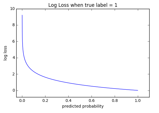
In the figure, we can see if we would get high loss if the predicted probability is far from the actual label (e.g., 0) and low loss if the predicted probability is close to the actual label (e.g., 0.9 and 1.0).

We need to convert the labels to categories (i.e., one-hot encoding) using the to_categorical function from tensorflow.keras.utils. The function takes an input array of integers and converts it to a one-hot encoded array.

class_labels = [0,1,2,0,2,1]
encoded_labels = to_categorical(class_labels)
print(encoded_labels)

In the output each component of the row is 0 except for the one corresponding to the label category. For example, in row 1, the label is 0, so the first component is 1 and the rest are 0. In row 2, the label is 1, so the second component is 1 and the rest are 0. In row 3, the label is 2, so the third component is 1 and the rest are 0.

[[1. 0. 0.]
 [0. 1. 0.]
 [0. 0. 1.]
 [1. 0. 0.]
 [0. 0. 1.]
 [0. 1. 0.]]

The example workflow with 5 predictors and 3 classes is shown below:

import pandas as pd
from tensorflow.keras.utils import to_categorical

df = pd.read_csv('mydata.csv') # load dataset
df.response = pd.Categorical(df.response) # convert response to categorical
df.response = df.response.cat.codes
y = to_categorical(df.response) # convert response to one-hot encoding

model = Sequential() # instantiate model

model.add(Dense(48, input_shape=(5,), activation='relu')) # add input and hidden layer
model.add(Dense(24, activation='relu')) # add another hidden layer
model.add(Dense(12, activation= 'relu' )) # add another hidden layer
model.add(Dense(3, activation='softmax')) # add output layer (3 classes)

model.compile(loss='categorical_crossentropy', 
  optimizer='adam', 
  metrics=['accuracy']) # compile model

# then train, evaluate, predict etc.

Multi-label Classification

As opposed to the multi-class classification, where each observation can only belong to one class, in the multi-label classification, each observation can belong to multiple classes (not mutually exclusive). So each label is independent of each other, and has their own probabilities between 0 and 1 (i.e., the sum of probabilities is no longer equal to 1). Thus, the output layer should have a sigmoid activation function. It’s like you are performing several binary classification problems for each label.

model.add(Dense(4, activation='sigmoid'))
model.compile(loss='binary_crossentropy', optimizer='adam', metrics=['accuracy'])

Convolutational Neural Network

Makes image classification feasible by:

• Reducing the number of input nodes
• Tolerating small shifts in where the pixels are in the image
• Taking advantage of the correlations in complex images

It does so by:

• Applying a Filter (Kernel) to the input image (usually a 3x3 pixels). The intensity of the filter is determined by the Backpropagation)

• Multiply image with the filter and sum the result to get a Dot product. Computing the Dot Product between the image and the filter, we say that the filter is convolving over the image (hence the name Convolutional Neural Network)
• Add a Bias to the result of the dot product to get a Feature Map
• Each value in the feature corresponds to the group of neigboring pixels the feature map captures any correlations in the image
• We apply an Activation Function to the feature map to get another Feature Map. The activation function is usually the ReLU function, resulting in all positive values.
• The feature map is run through another filter to get only the maximum value (aka Max Pooling), the filter run through the image but doesn’t overlap itself like the first filter
• Pooled layer converted to a vector of Input Nodes
• The input nodes are then plugged into the nodes like a regular Neural Network

Batch normalisation in Keras

Parameters/decisions that affect performance

How to determine the number of neurons in a deep learning neural network?

Determining the number of neurons in a deep learning neural network can be a challenging task and usually requires some experimentation and tuning to achieve good performance. Here are some general guidelines that can help in determining the number of neurons:

Input Layer: The number of neurons in the input layer is determined by the number of features in the input data. For example, if you have an image classification problem where each image is 28x28 pixels, the input layer should have 28x28 = 784 neurons.

Output Layer: The number of neurons in the output layer is determined by the number of classes in the problem. For example, if you have a binary classification problem, the output layer should have 1 neuron, and if you have a multi-class classification problem with 3 classes, the output layer should have 3 neurons.

Hidden Layers: The number of neurons in the hidden layers is determined by the complexity of the problem and the amount of data available for training. A common approach is to start with a small number of neurons and gradually increase the size of the hidden layers until the performance of the model starts to plateau.

Rule of thumb: A common rule of thumb is to use a number of neurons between the size of the input layer and the output layer. For example, if you have 784 input neurons and 10 output neurons, you can start with a number of neurons between 784 and 10 in the hidden layers.

Regularization: Adding regularization techniques such as dropout or L2 regularization can help prevent overfitting and allow you to use larger neural networks with more neurons.

In practice, the optimal number of neurons for a specific problem depends on various factors such as the size and complexity of the data, the number of classes, the number of hidden layers, and the regularization techniques used. Therefore, it’s recommended to start with a small number of neurons and gradually increase their size until you achieve good performance on your validation data.

Which activation function to use?

No magic formula, depends upon the problem. ReLU is the most popular activation function, but it is not always the best. Sigmoids not recommended for deep models, as they saturate and kill gradients. Tune with experiments. If the models run fast and you have a lot of data, you can try different activation functions and compare the performance. e.g., by using plots like this:

img source: ResearchGate